Navigation :

FIFO inventory method

The FIFO (first-in, first-out) inventory method implies that the first goods purchased are also the first goods to be sold. FIFO inventory can be seen as a theoretical model of the actual flow of goods, used for accounting or financial purposes. FIFO inventory can also be considered as a supply chain practice, intended to limit expiration or obsolescence issues that negatively impact stocked goods. FIFO inventory analysis allows to compute the stock “age” as well as to identify slow moving or dead inventory. In the following, we see how the FIFO analysis is carried out in practice, and also outlines the limits, both theoretical and practical, of this approach.

Table of contents

Physical FIFO

From a supply chain perspective focusing on the actual flow of goods, it is usually considered to be a good practice to have the earliest purchased goods shipped first. By adhering to this process, companies can typically mitigate most expiration write-off as long as the goods are not overstocked. This practice can also limit minor goods obsolescence associated with long storage periods (e.g. tarnished packaging).

For example, in fashion e-commerce, product returns may represent close to 50% of all goods being shipped. In this context, it is frequently considered as a best practice to first reship the goods that have been previously returned. This rule is an extension of the FIFO method, with the returns properly being taken into account. This method facilitates dealing with secondary sales channels at the end of a product collection.

Many warehouse systems do not differentiate at all as to which units get shipped, and ship a random unit of stock instead of the oldest one. The analysis of this practice goes beyond the scope of this document.

FIFO analysis

Unlike the physical FIFO, the FIFO analysis adopts a theoretical perspective on inventory, assuming that the earliest purchased units are shipped first, irrespective of the actual physical flow of goods. The FIFO perspective greatly simplifies the financial analysis of inventory.

In practice, all it takes to perform a FIFO analysis is:

the current stock levels
the history of purchase orders with delivery dates

Based on this data, FIFO analysis provides a way to compute the following:

inventory valuation, taking into account varying purchase prices
expected gross margin, which depends on the purchase prices
average inventory age (and extremes too)

In the following section, we illustrate how the above can be computed from a practical perspective.

Envision and FIFO analysis

Envision provides a fifo() function that is precisely dedicated to the FIFO analysis. Intuitively, given the current stock levels and past purchase orders, the fifo() method would be expected to return, in one way or another, a detailed composition of stock, indicating the age of each unit left in stock. It turns out that each unit is associated with one - and exactly one - purchase order line. This insight is a bit subtle, but it yields a method that consists of computing, for each purchase order line, how many units are still unsold considering the current stock levels.

Consequently, it is straightforward to see how these unsold quantities can be used for deriving the relevant financial KPIs. Let’s see how the fifo() function actually computes the unsold quantities associated with each purchase order line:

read "/sample/Lokad_Items.tsv" as Items[id] with
  Id : text
  StockOnHand : number
read "/sample/Lokad_PurchaseOrders.tsv" as PO expect [Id, Date] with
  Id : text
  Date : date
  "Quantity" as Qty : number

PO.Unsold = fifo(Items.StockOnHand, PO.Date, PO.Qty)
show table "Unsold" with
  Id
  PO.Date
  PO.Unsold

The script above begins by reading two files: the list of items and the list of purchase orders, as obtained from the sample dataset. Then, on line 5, a call to the fifo() function is performed. This function takes three arguments:

the current stock level
the date of the purchase order, typically the delivery date
the quantity associated with the purchase order

On line 6, the show table statement displays the results of the calculation.

Inventory Valuation

Inventory valuation is straightforward to compute with the following script:

read "/sample/Lokad_Items.tsv" as Items[id] with
  Id : text
  StockOnHand : number
read "/sample/Lokad_PurchaseOrders.tsv" as PO expect [Id, Date] with
  Id : text
  Date : date
  "Quantity" as Qty : number
  NetAmount : number

PO.Unsold = fifo(Items.StockOnHand, PO.Date, PO.Qty)
Items.StockValue = sum(PO.Unsold * PO.NetAmount / PO.Qty)

show scalar "Total stock value" with
  sum(Items.StockValue)

The script above multiplies the unsold quantity PO.Unsold by the original purchase unit price, computed as PO.NetAmount / PO.Qty.

Averaged Purchase Price

The purchase price can be averaged using the FIFO method. The script below is a variant of the previous one tailored for this purpose:

read "/sample/Lokad_Items.tsv" as Items[Id] with
  Id : text
  Name : text
  StockOnHand : number
read "/sample/Lokad_PurchaseOrders.tsv" as PO expect [Id, Date] with
  Id : text
  Date : date
  "Quantity" as Qty : number
  NetAmount : number

PO.Unsold = fifo(Items.StockOnHand, PO.Date, PO.Qty)
Items.StockValue = sum(PO.Unsold * PO.NetAmount / PO.Qty)
Items.PP = Items.StockValue /. sum(PO.Unsold)

where Items.PP > 0 // filter items without purchase orders
  show table "Purchase prices" with
    Id
    Items.Name
    Items.PP

The vector PP contains the purchase prices for all items. As we are using the /. division operator (which returns zero if the denominator is zero), all items where no purchase price can be computed are filtered on line 9 due to the lack of corresponding purchase orders.

Stock age

The stock age is also relatively straightforward to compute, however, it requires one extra ingredient: the date reflecting the present. Inventory data might sometimes be a few days old, and the current calendar date might not be the correct date for performing the analysis. In the example below, we introduce a variable named `today` which can be further adjusted in a real-life situation.

read "/sample/Lokad_Items.tsv" as Items[Id] with
  Id : text
  Name : text
  StockOnHand : number
read "/sample/Lokad_PurchaseOrders.tsv" as PO expect [Id, Date] with
  Id : text
  Date : date
  "Quantity" as Qty : number

// last observed date in data
today = max(PO.Date) + 1

PO.Unsold = fifo(Items.StockOnHand, PO.Date, PO.Qty)
PO.Age = (today - PO.Date) // age in days
Items.Age = sum(PO.Unsold * PO.Age) /. sum(PO.Unsold)

show table "Stock age" with
  Id
  Items.Name
  Items.Age
  order by Items.Age desc

The script above displays the list of all items in stock sorted by stock age, placing the oldest items at the top of the list. This calculation is performed on lines 8-10, averaging the age of each purchase order against its unsold quantities.

Limits of FIFO analysis

The expressiveness of the FIFO analysis comes from its underlying assumptions about the inventory flow. However, when data or the actual physical flow of goods diverge from these assumptions, the quality of the results tends to suffer. In this section, we review the most commonly encountered issues associated with FIFO analysis.

Truncated purchase history

While it might not be required to have the full purchase history since the beginning to carry out an accurate FIFO analysis, it is frequent that the oldest stocked units are present in stock for longer than the available depth of purchase history. Although in some industries, like aerospace, having 10 year-old parts is not uncommon, extracting 10 years’ worth of purchase history from company systems can be a tough challenge.

Stock-out replays are hazardous

If both the purchase order history and the sales order history are available, then it might be tempting to consider that the full history of stock-outs can be recomputed by replaying the whole sequence of purchase and sales orders in chronological order. In theory, through such a simulation, all inventory levels at any point in time could be re-computed, hence flagging all the periods where inventory levels were at zero as stock-outs.

Unfortunately, Lokad’s experience indicates that this approach almost never works. In this case, the slightest inventory discrepancy - such as a single unit not accounted for - wreaks havoc on the whole analysis because the periods of stock-out will almost never be at zero, but will rather consist of small quantities (positive or negative) which cannot be used to positively identify stock-outs.

Serial inventory

When all units have a unique serial number, and when all inventory movements are identified at the level of this serial number, then, the FIFO analysis should usually be considered as a very rough approximation. If the inventory is worth being physically tracked at the serial number (S/N) level, then this inventory is most certainly worth being analyzed by leveraging the extra level of detail provided by serial numbers.

Matching of sequences of events

Envision provides also an assoc.quantity() function that allows to match sequences of chronologically ordered quantitative events by linking two data sets. Possible use cases include assigning sold units (Orders) to purchased units (Purchase Orders Deliveries) with FIFO assumption with an objective of a margin analysis in multi-sourcing and evolving buy prices context, or assigning received unserviceable parts to shipped serviceable parts with LIFO assumption especially useful in an aerospace supply chain.

Hands-on illustration

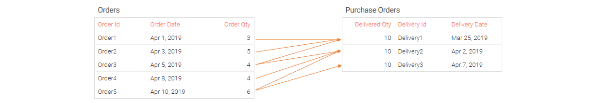
In the present sub-section, we describe the first use case, i.e. how an assoc.quantity() function assigns sold units to purchased units with FIFO assumption. We will be drawing information from two main files:

the history of orders with sales dates.
the history of purchase orders with delivery dates.

For each line stored in the Orders file (see the table on the left), an assoc.quantity() function identifies the corresponding line(s) in the Purchase Orders data set (see the table on the right) with the corresponding quantities. Each order line can initially be matched with any delivery line as presented below:

The Envision code reads as follows:

read "/sample/Lokad_Items.tsv" as Items[Id] with
  Id : text
read "/sample/Lokad_Orders.tsv" as Orders expect [Id, Date] with
  Id : text
  OrderId : text
  Date : date
  "Quantity" as OrderedQty : number
read "/sample/Lokad_PurchaseOrders.tsv" as PO expect [Id, Date] with
  Id : text
  "Quantity" as DeliveredQty : number
  "DeliveryID" as PONumber : text
  "DeliveryDate" as Date : date

PO.Rank = rank() by Id scan -PO.Date
Orders.POCount = count(PO.*) by Date

//The assoc.quantity() function is usually called with a table built using an extend.range() function.
table T = extend.range(Orders.POCount)

//SaleIdentifier and PurchaseIdentifier should be unique.
T.SaleIdentifier = concat(Id, "_", Orders.OrderId)
T.SoldQty = Orders.OrderedQty
T.SaleDate = Orders.Date
T.PurchaseIdentifier = same(concat(Id, "_", PO.PONumber)) by [Id, PO.Rank] at [Id, T.N]

T.PurchasedQty = same(PO.DeliveredQty) by [Id, PO.Rank] at [Id, T.N]
T.PurchaseDate = same(PO.Date) by [Id, PO.Rank] at [Id, T.N]
T.PurchaseRank = same(PO.Rank) by [Id, PO.Rank] at [Id, T.N]

T.AssociatedQuantity = assoc.quantity(T.SaleIdentifier, T.SoldQty, T.PurchaseIdentifier, T.PurchasedQty)
                       sort [T.SaleDate, T.PurchaseDate]

where T.AssociatedQuantity > 0
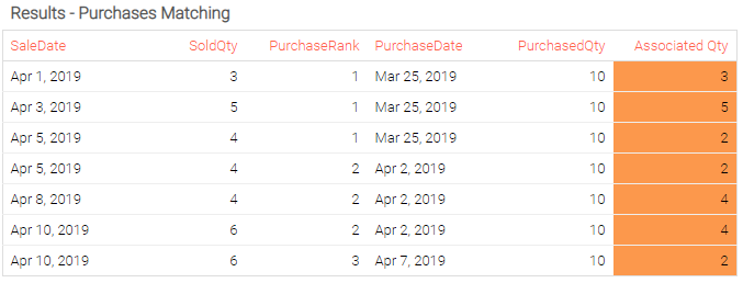
  show table "Results - Purchases Matching" with
    T.SaleDate
    T.SoldQty
    T.PurchaseRank
    T.PurchaseDate
    T.PurchasedQty
    T.AssociatedQuantity as "Associated Qty" {textColor:"tomato"}
    order by [T.SaleDate, T.PurchaseDate]

SaleIdentifier and PurchaseIdentifier should be unique. Identifiers are concatenations of multiple fields to ensure the unicity, e.g., OrderId is generally not enough to identify an Order line as it can be shared between several lines with different ordered items. If the ordered quantities of distinct items within one particular Order Id are different, assoc.quantity() will break. If ordered quantities of various items are the same, assoc.quantity() will not break, yet, it will return wrong results as it will assume that it is dealing with the same order line.

To simplify the use case, we present the algorithm behind the assoc.quantity() function assuming that there is only one item:

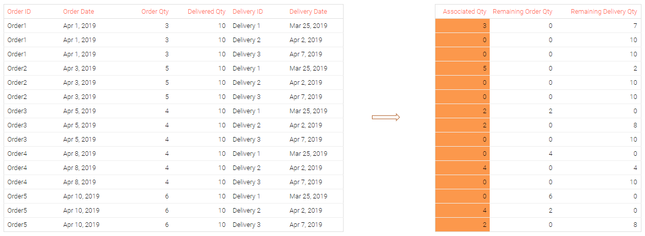
All these steps lead us to the following results:

Performance considerations

The assoc.quantity() function is usually called with a table built using an extend.range() function. This table is a Cartesian product of two existing tables, that are usually of significant size. The size of the product table could be a problem from a performance point of view (memory overflow and/or script failure risk). In addition, the logic behinds the assoc.quantity() function assumes a high quality of input data. If some data lines are missing in one of the input tables, it could lead to incorrect matching that will impact the analysis being performed.

User Contributed Notes

0 notes + add a note