Demand over lead time

This script illustrates a probabilistic demand forecasts (ISSM) along with the selection of the total demand integrated over a static horizon segment.

Check this script on the playground

/// Illustration of the demand integrated over the lead time

present = date(2021, 8, 1)
keep span date = [present .. date(2021, 10, 30)]
 
Day.Baseline = random.uniform(0.5 into Day, 1.5) // 'theta'
alpha = 0.3
level = 1.0 // initial level
minLevel = 0.1
dispersion = 2.0
 
Day.Q = each Day scan date // minimal ISSM
  keep level
  mean = level * Day.Baseline
  deviate = random.negativeBinomial(mean, dispersion)
  level = alpha * deviate / Day.Baseline + (1 - alpha) * level
  level = max(minLevel, level) // arbitrary, prevents "collapse" to zero
  return deviate
 
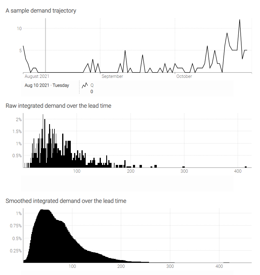
show linechart "A sample demand trajectory" a1d3 with Day.Q

L = 7 + poisson(5) // Reorder lead time + supply lead time

montecarlo 500 with
  h = random.ranvar(L)

  Day.Q = each Day scan date // minimal ISSM
    keep level
    mean = level * Day.Baseline
    deviate = random.negativeBinomial(mean, dispersion)
    level = alpha * deviate / Day.Baseline + (1 - alpha) * level
    level = max(minLevel, level) // arbitrary, prevents "collapse" to zero
    return deviate

  s = sum(Day.Q) when (date - present <= h)
  sample d = ranvar(s)

show scalar "Raw integrated demand over the lead time" a4d6 with d
show scalar "Smoothed integrated demand over the lead time" a7d9 with smooth(d)

The provided Envision script is an illustration of working with a probabilistic demand forecast in a supply chain context. It serves as an example to showcase the Envision syntax and its capabilities for demand forecasting and lead time analysis.

The script starts by defining the time period of interest (keep span date) and initializes parameters and variables for the minimal Innovation State Space Model (ISSM). The minimal ISSM in this script uses a single ’level’ parameter, making it simpler than variants that include seasonal factors, trends, etc.

The Day.Q calculation block iterates through each day (each Day scan date), updating the level variable using a combination of the current demand deviation and the previous level. The level is then used to calculate the mean demand, which is subjected to a negative binomial distribution to generate the demand deviation (deviate). The level variable is also constrained to a minimum value (minLevel) to prevent “collapse” to zero.

The script proceeds with a Monte Carlo simulation, iterating the demand calculation 500 times to accumulate 500 observations. The purpose of the Monte Carlo simulation is to account for the uncertainty in demand by simulating the random variables in the model. In this case, the random variables are the reorder lead time (L) and the supply lead time.

For each iteration, the same Day.Q calculation block is used as before, but with the additional constraint that the demand is only considered if the date minus the present date is less than or equal to the random lead time variable (h). The sum of the demands (s) within this constraint is collected in the sample d variable using the accumulator ranvar(s).

The script concludes by displaying a line chart of the sample demand trajectory (Day.Q) and two scalar values: the raw integrated demand over the lead time and the smoothed integrated demand over the lead time. The raw integrated demand is the direct output of the Monte Carlo simulation, while the smoothed integrated demand applies a smoothing function to the raw demand to provide a less noisy estimate.

Overall, this script demonstrates how Envision can be used for probabilistic demand forecasting and lead time analysis with a minimal ISSM approach, incorporating both a deterministic and a Monte Carlo simulation to capture the uncertainty in the supply chain.