Ranvars and Zedfuncs
Ranvars and zedfuncs are two advanced data types supported by Envision respectively intended to represent probability distributions and economic score functions. As there is a shared intent behind these two data types we present them together, although technically it would also be possible to introduce them separately. A joint presentation is also the opportunity to outline the numerous symmetries that exist between these two data types.
Table of contents
Overview
The first three points of the Quantitative Supply Chain Manifesto are:
- All possible futures must be considered; a probability for each possibility.
- All feasible decisions must be considered; possibilities vs. probabilities.
- Economic drivers must be used to prioritize feasible decisions.
This vision has proved to be the cornerstone of most of Lokad’s supply chain achievements. However, it raises many questions: how should probabilities be represented? How should decisions be represented? How to manage the coupling between a decision and its uncertain economic outcome? Executing this vision with classical tooling - i.e. capabilities that a spreadsheet could provide - is challenging to say the least. The number of probabilities to be considered is large, which makes naive approaches somewhat computationally intractable. The expression of the coupling of probabilities and of economic outcomes proves difficult. Finally, naive implementations steer initiatives toward fragile and buggy codebases.
The two algebras of ranvars and zedfuncs represent Lokad’s technological answer to support this vision. The term ranvar stands for random variable, while zedfunc stands for $\mathbb{Z}$ functions where $\mathbb{Z}$ is the integer set (both positive and negative). Ranvars and zedfuncs are two specialized data types in Envision that have their own respective algebras, with operators like + (add) and * (multiply). Ranvars represent probability distributions over $\mathbb{Z}$ while zedfuncs represent functions $\mathbb{Z} \to \mathbb{R}$. The combination of these two algebras provide (arguably) elegant solutions to entire classes of inventory problems (replenishment, purchasing, stock rebalancing, etc).
Ranvars are typically used to represent probabilistic forecasts such as future demand, future lead times, future package returns, future production yields, etc. Indeed, when looking at the future, the uncertainty is irreducible. Instead of dismissing the uncertainty, Lokad proposes to instead embrace this notion, and introduces ranvars as a tool to address this requirement. Unlike the traditional “multiple-scenarios” perspective, ranvars offer a base mechanism to deal with all future scenarios at once.
Zedfuncs are used to represent the economic reward (or loss) associated with unidimensional options (i.e. potential decisions), typically quantities for a SKU to be ordered, produced, moved, discarded, etc. Instead of narrowing down options to a single number, we leave the options open. For example, unlike a traditional min/max inventory policy, a zedfunc allows you to simultaneously consider all the outcomes for every single reordered quantity (+0 unit, +1 unit, +2 units, etc). Zedfuncs offer a base mechanism to deal with all options.
Both ranvars and zedfuncs behave like generalized numbers in a way. Mathematically-inclined minds could observe that ranvars and zedfuncs operate respectively in their own (quasi) vector space. More casually, we can say that the basic arithmetic operations available for numbers - addition, subtraction, multiplication - also happen to be available for both ranvars and zedfuncs, although they mean something different. Furthermore, both ranvars and zedfuncs can be combined (via addition or multiplication) with a regular number as well.
A ranvar represents a random variable $X$ where the possible outcomes - usually denoted $\Omega$ - is $\mathbb{Z}$ and where the probabilities are real, nonnegative numbers. It can be seen as a function $p:\mathbb{Z} \to \mathbb{R^+}$ where $p(x) = P(X = x)$ and where $p$ satisfies $$\forall x \in \mathbb{Z}, p(x) \ge 0$$ and $$\sum_{x \in \mathbb{Z}} p(x) = 1$$
A zedfunc represents a function $f: \mathbb{Z} \mapsto \mathbb{R}$. Unlike a ranvar, the values taken by the function are not obligated to be positive, and the sum over $\mathbb{Z}$ is not expected to be bounded either.
The following Envision script illustrates how a ranvar and a zedfunc can be generated and plotted:
R = poisson(13)
show scalar "My Ranvar" a1b2 with R
Z = linear(2)
show scalar "My Zedfunc" a3b4 with Z
The function poisson() returns a Poisson probability distribution of parameter $\lambda=13$. The function linear() returns a function $x \mapsto 2x$. Two scalar tiles are used to display the two values respectively.
One of Envision’s most interesting capabilities of the twin algebras of ranvars and zedfuncs is the capacity to turn a ranvar into a zedfunc when given a few economic parameters. In other words, to turn probabilities into economic outcomes of decisions. Let’s illustrate this idea to make it less obscure.
Let’s consider a situation where, for a given SKU, the total future demand to be served over the next lead time is denoted D. As the future is uncertain, D is a probability distribution reflecting the probability of observing each level of demand over the lead time. Let u be the per-unit stock-out penalty cost for not servicing 1 unit of demand. Let S be the marginal stock penalty associated with each stock position. The following script computes S:
D = poisson(3)
u = -2
S = stockrwd.s(D) * u
show scalar "Stockout penalty" a3b4 with S
In the above script, the demand D is modeled as a Poisson distribution of mean 3. The stockout penalty is set at -2 (negative because it’s a penalty). Finally, the stockout component of the special stock reward function stockrwd.s() is used to compute S.
The chart plotting S can be interpreted as follows: we have S(0) = -6 because it corresponds to the expected loss (-2 per unit) associated to the stock position zero, where none of the unit of the demand will be serviced (the mean of the demand is 3). We have S(1) ≈ 1.9 because there is a very high probability that the demand will be at least one unit. Hence, the marginal contribution of the first unit in stock is close to 2, but still smaller than 2. We have S(2) ≈ 1.6 which is lower than S(1) because the probability that the demand will be at least two units is still high, but lower than “at least one unit”. The stock reward function is complex, we will revisit this function in a later section.
Historical note: Early on, Envision had neither ranvars nor zedfuncs. Thus, supply chain scientists were extensively relying on extend.range() instead, through a process that was internally referred to as building “grids”. It’s the same “grid” term as found in Quantile Grids which was our 3rd generation forecasting approach. However, while this approach had the merit of frontally - albeit crudely - tackling the uncertainty angle, most operations were cumbersome to write. Furthermore some operations, like convolutions (see below), could only be barely approximated. Ranvars and zedfuncs remove almost entirely the need to resort to grids, except at the very end of the process, typically when building a prioritized list of decisions of some kind.
Basic operations on ranvars
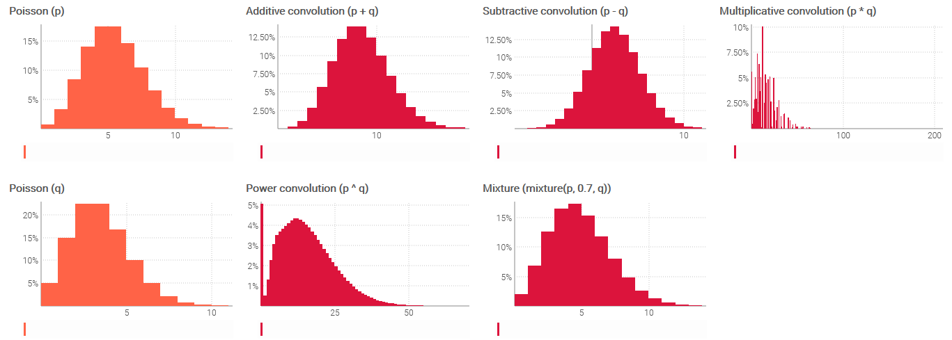
The arithmetic operations between ranvars can be interpreted as operations between independent random variables. The following script illustrates those operations:
X1 = poisson(5)
X2 = poisson(3)
show scalar "Addition" a1c3 with X1 + X2
show scalar "Subtraction" d1f3 with X1 - X2
show scalar "Multiplication" a4c6 with X1 * X2
show scalar "Power" d4f6 with X1 ^ X2
show scalar "Mixture" a7c9 with mixture(X1, 0.5, X2)
In the above script X1 and X2 represent two independent Poisson random variables of respective means of 5 and 3. The operations that follow illustrate the series of arithmetic operations available for ranvars.
More generally, the following table outlines the interpretation to be given to each one of those operations.
| Operation | Formula |
|---|---|
| Addition. If $X_1$ is the production lead time and $X_2$ is the shipping lead time, then $X_1+X_2$ is the duration of both production and shipping. | $P(X_1 + X_2 = x) = $ $\sum_{x_1 + x_2 = x} P(X_1 = x_1)P(X_2 = x_2)$ |
| Subtraction. If $X_1$ are future shipments and $X_2$ are future returns for a given time period, then $X_1-X_2$ is the net flow good for the period. | $P(X_1 - X_2 = x) =$ $\sum_{x_1 - x_2 = x} P(X_1 = x_1)P(X_2 = x_2)$ |
| Multiplication. If $X_1$ is the future number of basket sold and $X_2$ is the future number of items in each basket then $X_1 * X_2$ is the future number of items sold. | $P(X_1 * X_2 = x) =$ $ \sum_{x_1 * x_2 = x} P(X_1 = x_1)P(X_2 = x_2)$ |
| Power (a). If $X$ is the future daily demand (assumed stationary) and $Y$ is the future lead time in days then $X ^ Y$ is the future total demand over the duration of the lead time. | See the reference documentation. |
| Mixture. If $X_1$ is the transport lead time by air and $X_2$ is the transport lead time by sea and there is a 50/50 chance that transport will happen by sea or by air, then $\texttt{mixture}(X_1,X_2)$ is the expected transport lead time. | $P(\texttt{mixture}(X_1,X_2)=x) = $ $\frac{1}{2}P(X_1=x)+\frac{1}{2}P(X_2=x)$ |
Under the hood, when ranvars are involved, the calculations performed by Envision are typically convolutions. These operations require a lot more computing resources than mere number additions or multiplications. Nevertheless, the Lokad platform is designed to execute a large number of these operations, in a distributed fashion if needed, as required by supply chain scenarios.
Integers can be “plunged” into ranvars by re-interpreting them as a Dirac random variable where the entire probability mass is concentrated on a single outcome. This happens to be the position adopted by Envision. When combining, in a single operation, both a number and a ranvar, the number is first converted to a Dirac random variable and then the operation proceeds as usual. This mechanism is illustrated by:
X1 = poisson(5)
X2 = 3
show scalar "Addition" a1c3 with X1 + X2
show scalar "Subtraction" d1f3 with X1 - X2
show scalar "Multiplication" a4c6 with X1 * X2
show scalar "Power" d4f6 with X1 ^ X2
show scalar "Mixture" a7c9 with mixture(X1, 0.5, dirac(X2))
The script above is almost identical to the previous one. The only difference is the variable X2, which is replaced by a number. This script is strictly equivalent to the following one:
X1 = poisson(5)
X2 = dirac(3)
show scalar "Addition" a1c3 with X1 + X2
show scalar "Subtraction" d1f3 with X1 - X2
show scalar "Multiplication" a4c6 with X1 * X2
show scalar "Power" d4f6 with X1 ^ X2
show scalar "Mixture" a7c9 with mixture(X1, 0.5, X2)
In the above script, the function dirac() generates a Dirac random variable associated with the integer 3. The function dirac() rounds its sole number argument to the nearest integer prior to generating the random variable.
Basic operations on zedfuncs
The arithmetic operations between zedfuncs can be interpreted as vector operations over $\mathbb{Z} \to \mathbb{R}$ . The following script illustrates these operations:
f = linear(2) - 2   // f(x) -> 2x - 2
g = linear(-1) + 3  // g(x) -> 3 - x
show scalar "Addition" a1c3 with f + g
show scalar "Subtraction" d1f3 with f - g
show scalar "Multiplication" a4c6 with f * g
The function linear returns a zedfunc defined by $x \mapsto ax$ where $a$ is the number passed as argument. More generally, the following table outlines the interpretation to be given to each one of those operations.
| Operation | Formula |
|---|---|
| Addition. If $f$ is the carrying cost for every stock position related to stock obsolescence and $g$ is the insurance cost for every stock position, then $f+g$ is the sum of those costs. | $f + g : x\mapsto f(x) + g(x)$ |
| Subtraction. If $f$ is the expected margin for every stock position, and $g$ is the carrying cost for every stock position, then $f-g$ is the next reward margin minus cost. | $f - g : x\mapsto f(x) - g(x)$ |
| Multiplication. If $f$ is the expected number of serviced units for every stock position, and if $g$ is the gross-margin on every stock position - shaped by price breaks - then $fg$ is the expected gross-margin by stock position. | $fg : x\mapsto f(x) g(x)$ |
Numbers can be “plunged” into zedfuncs by re-interpreting them as constant functions. This happens to be the position adopted by Envision. When combining, in a single operation, both a number and a zedfunc, the number is first converted to a constant function, and then the operation proceeds as usual. The mechanism is already at play in the above script, however it could have been written in a more explicit fashion with:
f = linear(2) - constant(2)   // f(x) -> 2x - 2
g = linear(-1) + constant(3)  // g(x) -> 3 - x
show scalar "Addition" a1c3 with f + g
show scalar "Subtraction" d1f3 with f - g
show scalar "Multiplication" a4c6 with f * g
The function constant returns the zedfunc defined by $x \mapsto a$ where $a$ is the number passed as an argument.
Precision, resolution and performance
A data structure capable of perfectly recording any arbitrary function $f:\mathbb{Z} \to \mathbb{R^+}$ (ranvar-like) or any arbitrary function $f:\mathbb{Z} \to \mathbb{R}$ (zedfunc-like) would need to potentially store an infinite amount of data. This option isn’t realistic and, thus, isn’t the path followed by Lokad. Instead, both ranvars and zedfuncs, as implemented by Lokad, are approximate data structures, both in resolution and precision.
An approximate resolution means that the value $f(x + \epsilon)$ can be approximated by $f(x)$ when $\epsilon \ll x$ (i.e. $\epsilon$ very small compared to $x$). The further away from zero, the lower the resolution both for ranvars and zedfuncs alike.
An approximate precision means that only the most significant bits of precision of $f(x)$ are preserved. The process is similar to rounding except that numbers aren’t rounded to a given number of decimals, but rounded to a given number of bits.
Lokad uses two distinct compression algorithms for ranvars and zedfuncs. These two algorithms differ by their intent. For ranvars, the goal of the compression is to preserve the local, absolute mass of probabilities. This property ensures that, for example, the probability associated with a tail event does not vanish, even if the resolution is relatively poor. For zedfuncs, the goal of the compression is to preserve the local variations. This property ensures that when facing a highly non-linear economic phenomenon, the “cliff” doesn’t get smoothed away.
These approximations are necessary to make ranvars and zedfuncs as predictable, as far as computing resources are concerned, as regular numbers. Keeping all workloads bounded and predictable is an essential feature of any system intended to support a supply chain’s daily operations.
Decomposing ranvars and zedfuncs
So far, we have seen multiple ways to compose complex ranvars and zedfuncs starting from “simple” numbers through their respective algebras, but those types also offer decomposition mechanisms to extract local values.
The function extend.ranvar() takes a vector of ranvars as an argument and returns a table that extends the original vectors containing boundaries of the underlying probability buckets within the ranvar.
x = poisson(3)
table G = extend.ranvar(x)
show table "poisson(3)" a1c5 with
  G.Min
  G.Max
  int(x, G.Min, G.Max) as "Probability"
The table G produced by extend.ranvar() contains two vectors named Min and Max, which represent the inclusive boundaries of buckets associated with the original ranvar. The function int(), which stands for integral, returns the probability of the segment identified by its inclusive boundaries.
The buckets returned by extend.ranvar() are contiguous, thus zero-probability buckets may be returned. On the extreme left and right, the buckets of zero probability are pruned. However, the segment [0, 0] is always returned by extend.ranvar(). This behavior is intended to facilitate the most common operations, which typically involve prioritized lists of decisions.
Conversely, a ranvar can be (re)composed using the function ranvar.buckets().
x = poisson(3)
table G = extend.ranvar(x)
G.P = int(x, G.Min, G.Max)
y = ranvar.buckets(G.P, G.Min, G.Max)
show scalar "Original" a1b3 with x
show scalar "Recomposed" c1d3 with y
Similarly, zedfuncs can also be decomposed via the valueAt() function.
f = linear(1) * linear(1) - 4
table T = extend.range(5)
show table "f(x)=x^2-4" a1b5 with
  T.N
  valueAt(f, T.N)
However, as zedfuncs typically don’t have well defined “support” segments, unlike ranvars, Envision does not include a counterpart to expose the underlying buckets and values.
Empirical ranvars
A common way of constructing ranvars is through empirical distributions, that is, the direct aggregation of observed values. This process is illustrated by:
table Observations = with
  [| as N |]
  [| 2 |]
  [| 3 |]
  [| 6 |]

p = ranvar(Observations.N)
q = smooth(p)
r = mixture(dirac(Observations.N))
s = mixture(poisson(Observations.N))

show scalar "Empirical" a1c3 with p
show scalar "Smoothed" d1f3 with q
show scalar "Mixture Dirac" a4c6 with r // identical to 'p'
show scalar "Mixture Poisson" d4f6 with s // identical to 'q'
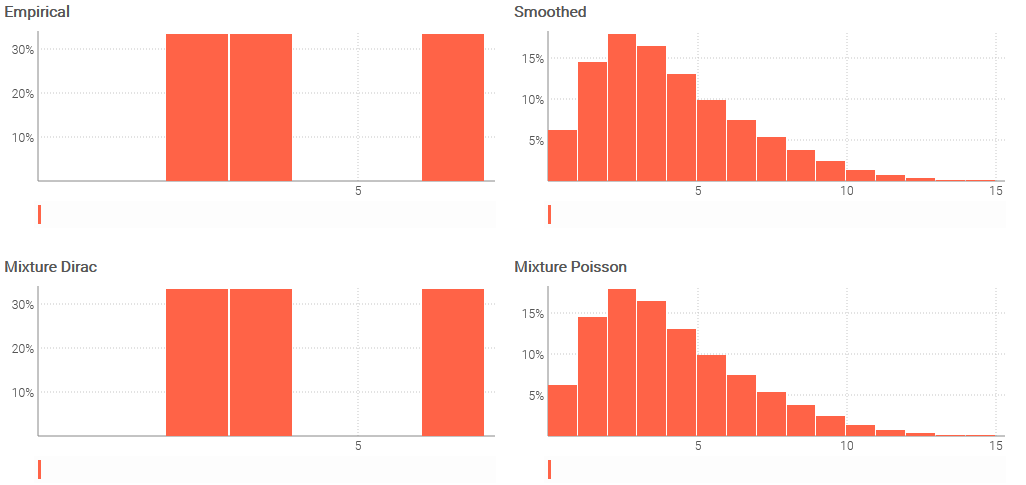
In the above script, the aggregator ranvar() takes numbers as input and returns a ranvar. Yet, when there are few observations, the empirical distribution can look excessively spiky and be unrepresentative of the real underlying distribution. Thus, the ranvar can be smoothed thanks to the function smooth(). Similary, the aggregator mixture() takes ranvars as input and returns the averaged ranvar.
The ranvar() aggregator can be seen as the application of an equi-weighted mixture of Dirac distributions obtained from the original observation though the function dirac(). This equivalence is illustrated above by p and r being numerically identical.
The smooth() function can be seen as as an weighted mixture of Poisson distributions where each Poisson distribution (associated to an integral mean) is weighted according to the probability of the mean. This equivalence is illustrated above by q and r being numerically identical.
The same empirical generation process can be revisited with weights in order to reflect a situation where the original observations would be associated to various biases.
table Observations = with
  [| as N, as Weight |]
  [| 2, 0.4 |]
  [| 3, 0.4 |]
  [| 6, 0.2 |]

p = ranvar(Observations.N, Observations.Weight)
q = smooth(p)
r = mixture(dirac(Observations.N), Observations.Weight)
s = mixture(poisson(Observations.N), Observations.Weight)

show scalar "Empirical" a1c3 with p
show scalar "Smoothed" d1f3 with q
show scalar "Mixture Dirac" a4c6 with r // identical to 'p'
show scalar "Mixture Poisson" d4f6 with s // identical to 'q'
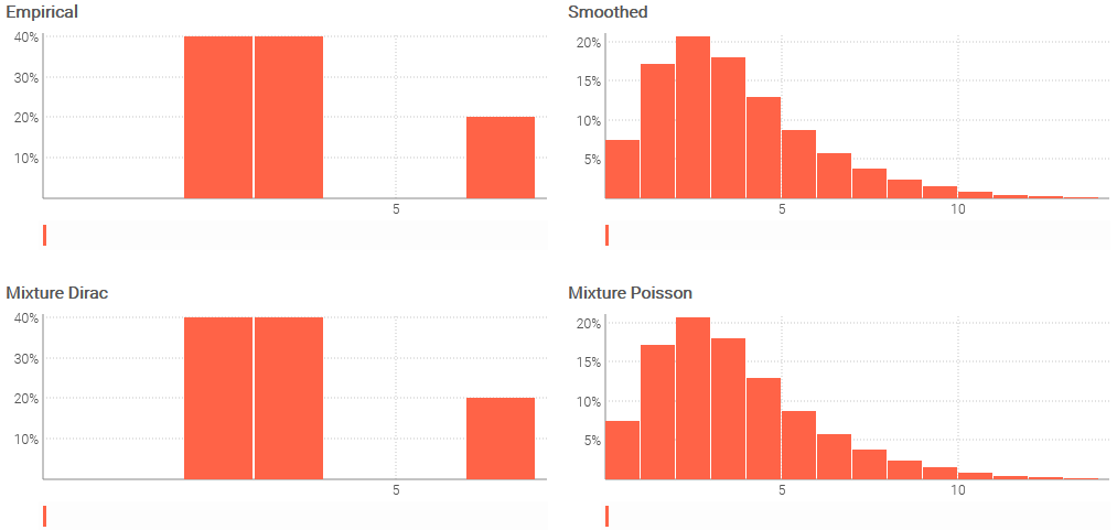
The above script is a variant of the previous one where weights are provided, first for the ranvar() aggregator and second for the mixture() aggregator (with two calls). Both aggregators takes two arguments, the input value and the weight. Weights are expected in the interval [0, 1] and are scaled back to 1 if the sum doesn’t add up to 1.
Handy ranvar invariants
The commutative, associative and distributive properties of convolutions benefit to the ranvar algebra. The following script illustrates some theoretical equivalences within Envision:
a = 3
b = 5
X1 = poisson(4)
X2 = poisson(2)

M = mean(X1 + dirac(a)) // is equal to
M = mean(X1) + a

S = (X1 ^ a) ^ b // is equal to
S = X1 ^ (a * b)

M = mean(X1 + X2)  // is equal to
M = mean(X1) + mean(X2)

V1 = variance(X1 + X2)  // is equal to
V1 = variance(X1) + variance(X2)

M1 = mean(X1 ^ dirac(a))  // is equal to
M1 = mean(X1) * a

V2 = variance(X1 ^ dirac(a))  // is equal to
V2 = variance(X1) * (a^2)
The choice of one among theoretically equivalent writings is important in terms of accuracy of the result. For example:
table T = with
  [| as R       |]
  [| poisson(1) |]
  [| poisson(3) |]
  [| dirac(2)   |]

A = sum(mean(T.R)) // 'A' is more accurate than 'B'
B = mean(sum(T.R))
As a rule of thumb, it’s best to keep working with plain numbers for as long as possible. This practice is superior in terms of numerical accuracy, but also in terms of compute performance.