Workshop #3: Distribution Network Analysis
This workshop is intended for Master students willing to learn more about Supply Chain Optimization using Lokad’s dedicated programming language “Envision”. Envision is dedicated to the predictive optimization of supply chains. A sample dataset is provided as well. The topic of this workshop will be the structure of a retail network including an online selling channel. Starting with an analysis of how the network is structured to understand precisely how the company serves customer demand, we will then dive into an analysis of the current stock levels. Finally, the use of supply chain quantitative tools will be carried out to identify actions to improve stock availability while minimizing costs at the same time. This workshop should take between 5 to 10 hours to complete, depending on your programming skills. No prerequisite from the two first workshops (#1 Supplier Analysis and #2 Sales analysis) is required. The full documentation to our programming language Envision is public and available on Envision Reference - Lokad Technical Documentation.

Table of contents
Introduction
Company overview
CM is a fictitious European company selling outdoor clothing with retail stores in three countries: Germany, France, and Italy. CM also has a strong online presence. The company’s website offers customers the ability to purchase their products online, with home delivery available for added convenience. In addition to their website, CM sells their products through various online platforms, such as Amazon and other e-commerce marketplaces. This allows CM to reach a wider audience and connect with customers who prefer to shop online.
The company was founded by a group of friends who were passionate about the outdoors and wanted to make quality outdoor clothing and sporting equipment more accessible to everyone.
The first store opened in Germany, and it was an instant success. The store was filled with high-quality outdoor clothing and equipment that was both stylish and functional. The founders of CM believe that people should be able to enjoy the outdoors without sacrificing style or comfort.
CM quickly expanded to other European countries, opening stores in France, and Italy. Each store has a unique style and atmosphere that reflects the local culture and environment. The stores are more than just retail spaces; they are community hubs where outdoor enthusiasts can come together to share their passion for adventure.
Distribution Network
Operating a distribution network for a company selling products both online and in physical stores across Europe presents a multifaceted challenge. The continent’s diverse markets, regulatory environments, and consumer preferences demand a complex and adaptive approach. Consumer expectations also vary across Europe. Online shoppers seek rapid, reliable delivery, while in-store customers expect a broad product selection and a seamless shopping experience. Balancing these diverse demands requires intricate inventory management and demand forecasting.
The company has one large warehouse that keeps stock distributed to the three points of sale located in three different European countries: France (Paris), Germany (Berlin) and Italy (Milan).
Recently and over the year 2022, CM has observed disruptions and its costs of storage have increased. Thus, the company has decided to tackle the issue and to better optimize its stock distribution across its network. Many products were either stocked-out or overstocked, penalizing the company capacity to serve demand from the other store or online.
Objectives of the Workshop
The goal of this session is to be able to describe the overall distribution network and identify the impact of poor inventory management by answering the following questions:
-
What is the supply chain structure?
-
Where is the stock located?
-
How is customer demand covered?
-
How internal lead times impact products availability?
-
What is the impact of a poor stock balance across the network? How can a good decision impact the company’s financial health?
The session will be structured in 3 steps:
-
The global network description.
-
An analysis of the current stock in the network.
-
Which actions can be taken to sanitize stock levels?
Useful Definitions
-
SKU: Acronym for Stock Keeping Unit, it corresponds to the unique reference of a product in its location.
-
Dispatch Leadtime: The dispatch (or transfer) lead time refers to the time it takes to get a transfer between two locations in the same network. It can be defined as a difference between Reception Date (
PO.DeliveryDate) and Order Date (Orders.Date) when the order is internal.
Hint: Envision adopts array programming, processing whole columns at once, like SQL. The . operator is used to specify the table and the column of that table, i.e. MyTable.MyField. All tables of the dataset are detailed in the next section called Dataset.
-
Net Amount: the total sales amount generated by a
Sales Orderline. It is the product of quantity sold and sell price:OrderQty * SellPrice. -
Margin: Measures how much profit is generated by a sale. It is defined as
SellPrice–BuyPrice. -
Stockout: usually an item is considered facing stockout when its stock level is not sufficient to serve all sales. There are many definitions of stockout periods, however in this workshop we will consider an item to be in stockout when its stock is 0.
-
Overstock: An item is considered overstocked when its stock level is too high, considering the demand it sees over a given period.
-
Carrying cost: You can read about different kinds of inventory carrying costs. For the purpose of this workshop we consider following model: carrying cost is equal to 20% of the item’s buy price over a year (52 weeks).
-
Return on Investment (ROI): a metric to quantify if considered decision is expected to be profitable or not. It considers the various costs and profit generated by a decision.
Dataset
The dataset provided for this workshop consists from 7 tables (see the data schema below). They are preloaded in the Envision playground (see lines of code #4 to #115).
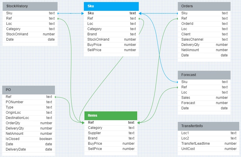
In this schema, blue and green arrows are indicating the relationships between the tables, specifically the foreign key to primary key relationships. These relationships are essential for joining tables in a relational database to query data across different entities.
For example, the Sku table, which stores information about stock keeping units, is a central table with relationships to the StockHistory, Orders, and Forecast tables through their foreign keys, as indicated by the blue arrows. This implies that the .Sku field in these tables references the primary key in the Sku table, allowing for a relational link between the data in these different tables.
The arrow lines start from the foreign key side with the arrowheads pointing towards the primary key side, which is a typical way to denote the direction of the relationship from the foreign key in one table to the primary key in another.
1. Items Table (Catalog.tsv)
- Purpose: Details each item sold by CM.
- Contents: Includes item reference, category, supplier, brand, and both buying and selling prices.
- Key Fields:
Ref(Item Reference),Category,Supplier,Brand,BuyPrice,SellPrice.
2. SKU Table (SKU.tsv)
- Purpose: Provides information at the SKU level, including stock and pricing details.
- Contents: Contains SKU, item reference, location, category, brand, stock on hand, and pricing.
- Key Fields:
Sku,Ref(Item Reference),Loc(Location),Category,Brand,StockOnHand,BuyPrice,SellPrice.
3. Orders Table (Orders.tsv.gz)
- Purpose: Records sales transactions to customers.
- Contents: Includes order ID, date, SKU, item reference, location, quantity delivered, net amount, client, and sales channel.
- Key Fields:
OrderId,Date,Sku,Ref(Item Reference),Loc(Location),DeliveryQty,NetAmount,Client,SalesChannel.
4. Purchase Orders Table (PurchaseOrders.tsv)
- Purpose: Tracks purchase orders, including both external supplier orders and internal transfers.
- Contents: Features PO number, dates, item reference, delivery details, order and delivery quantities, net amount, closure status, type, and locations.
- Key Fields:
PONumber,Date,Ref(Item Reference),DeliveryDate,OrderQty,DeliveryQty,NetAmount,IsClosed,Type,OriginLoc,DestinationLoc.
5. Stock History Table (StockHistory.tsv)
- Purpose: Provides a historical snapshot of stock levels for each SKU.
- Contents: Includes date, SKU, item reference, location, category, and stock on hand.
- Key Fields:
Date,Sku,Ref(Item Reference),Loc(Location),Category,StockOnHand.
6. Weekly Forecast Table (WeeklyForecast.tsv)
- Purpose: Offers sales and demand forecasts on a weekly basis.
- Contents: Contains date (week’s Monday), SKU, item reference, location, actual sales, and forecasted demand.
- Key Fields:
Date,Sku,Ref(Item Reference),Loc(Location),Sales,Forecast.
7. Transfert Info Table
- Purpose: Details the logistics and costs associated with internal transfers between locations.
- Contents: Includes origin and destination locations, transfer lead time, and unit cost.
- Key Fields:
Loc1(Origin),Loc2(Destination),TransfertLeadtime,UnitCost.
Part 1: Network Description
1. Questions
a. Points of sales
-
Display the historical sales repartition among the different selling channels in a barchart tile.
-
Which location(s) serve customer demand? Which types of markets are associated to each location (web/retail)?
b. Stocks
-
Display the current stock levels among the localizations in a piechart tile.
-
Which location(s) hold stock and how is the stock split between locations?
c. Purchase deliveries
-
Find the column in the Purchases Orders (
POtable) that differentiates purchase orders coming from suppliers and internal transfers. -
Display the historical stock on order value (coming from suppliers only) for each destination location in a
barcharttile. -
Which location(s) can receive POs from external suppliers?
d. Transfers
-
Display the historical stock in transit value for each couple [Origin Location, Destination Location] in a
barcharttile. -
Which transfers directions can be deduced within the network?
-
Display in a table tile the average transfer time between each couple [Origin Location, Destination Location]? This duration will be called the Dispatch Leadtime.
e. CM’s network description
Based on your answers above, how many layers are there in CM’s network? Draw a simplified version of the network that mentions:
-
Locations where there is customer demand and which selling channel is involved.
-
Locations where stock is held, and which transfers are allowed.
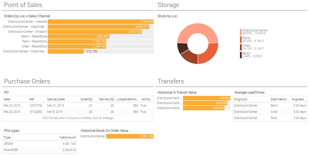
2. Conclusion
To effectively analyze and make informed decisions regarding CM’s supply chain, the initial and crucial step is to establish a comprehensive understanding of its supply chain structure and associated flows. This encompasses a clear comprehension of sales locations, marketplaces, stock levels, purchase orders, and transfer dynamics. By gaining a holistic view of how CM’s supply chain functions, one can strategically navigate and optimize its operations, ultimately leading to improved efficiency, cost-effectiveness, and the ability to provide superior service to customers. In essence, the foundation for successful supply chain management begins with a thorough grasp of its structure and intricacies.
Hint: To check yourself here is an example of a dashboard that you might built. The exact layout of the dashboard and colors might be different depending on your choices.
Part 2: Stock Analysis
1. Questions
a. Type of stock per location
-
To understand stocking CM organization, display the stock repartition per item’s category for each location in a treemap tile.
-
Are there one or several categories stocked only in specific locations?
-
Which factors might explain this observation?
b. Historical stockouts
- Which category is currently the most stocked-out on average?
Hint: define an availability flag per item to solve this question: if the item is in stock on a given day, its availability flag for this day is 1. Else it is 0.
-
i. For each month of 2022, display the availability rate of each category per location in a
tabletile.ii. Display the availability ratio at a weekly level for each location in 2022 using a linechart tile.
-
Are there any observable patterns when looking at the availability rates for the months of November and December? If yes, which reasons can explain these patterns?
-
i. Which SKU, having been sold at least once in 2022, had the most stock-outs over the year? You can display the results in a
tabletile.ii. To get a first estimation of the lost sales caused by the rupture of the SKU, display in a
linechart, over the year 2022, the sales and average forecast for the example identified just above.iii. For the same SKU, what is the shortfall in sales and margin over the year 2022?
Hint: to make a reasonable first estimation, you can use the average weekly forecast as the lost sales during a stock out period.
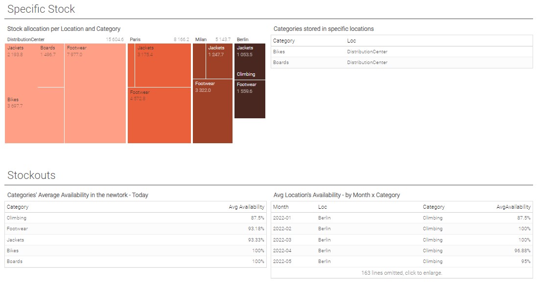
2. Conclusions
Stock Distribution
CM demonstrates distinct patterns of stock allocation across product categories and locations. This reveals a strategic approach to inventory management, with certain categories being predominantly housed in specific locations, driven by factors such as logistical considerations, storage capacity and targeted marketing.
Historical Stock Out Patterns
CM’s stock-out patterns provide insights into potential areas of improvement in stock management. This analysis unveils trends and underlying factors that influence stock-out incidents, enabling CM to make more informed decisions to address these challenges.
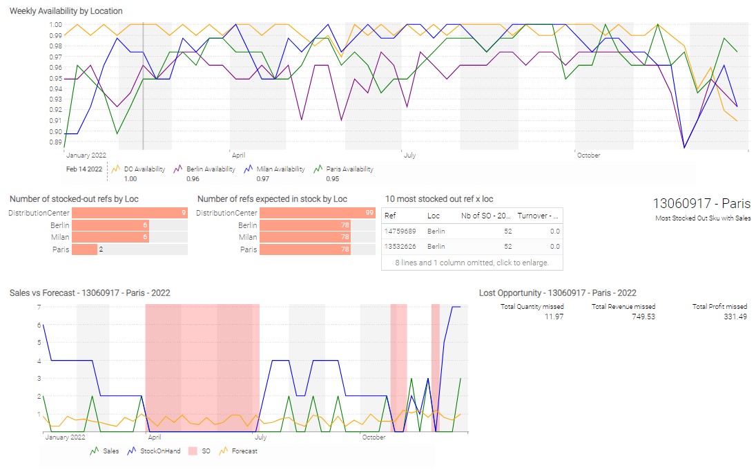
Impact of Stock outs
The analysis of references frequently experiencing stock-outs provides crucial insights into how these shortages affect CM’s sales and margins. This understanding is essential for assessing the real-world consequences of stock-outs on CM’s overall operational and financial performance.
Hint: To check yourself here is an example of a dashboard that you might built. The exact layout of the dashboard and colors might be different depending on your choices.
Part 3: Leverage Actions
1. Questions
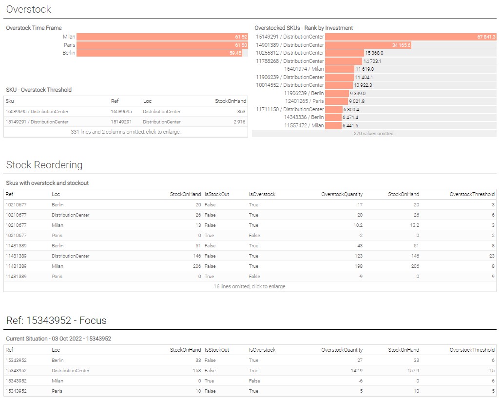
a. Overstock
We consider a product to be overstocked in one location if the stock available is above the stock needed to cover very high demand scenarios over one Dispatch Leadtime (see Part 1. D.) plus two Dispatch Periods. We’ll define this total duration as the Overstock Timeframe: Overstock Timeframe = Dispatch Leadtime + 2*Dispatch period.
The Dispatch Period corresponds to the duration between 2 possible dispatch decisions. The CM company carries out its transfers every 4 weeks from its central warehouse to its various branches. Regarding the Dispatch Leadtime, we will compute it as the average transfer time observed between the main warehouse and each location.
-
Estimate the duration of the Overstock Timeframe for each location. Display the results in a
barcharttile. -
We can define the surplus stock for a product as the stock exceeding the 95th quantile of its probabilistic demand over the Overstock Timeframe. Find all products currently overstocked using the probabilistic forecast given. Display the overstock value for each SKU in a
barchartby ranking them.
Hint: As a preliminary step, it is recommended to figure out the overstock threshold for each product. You can directly use the quantile function.
b. Stock Relocation
Let’s assume that the last transfer took place 7 days ago and that today is 2022/11/03.
Necessary and useful information:
-
No backorders: if no stock is available, sales to any customer are not possible.
-
We may want to transfer from one location the overstocked quantities to another location for which stocks may not be sufficient to cover customer demand.
-
We consider the storage cost as being equal to 20% of the item’s buy price over a year (52 weeks). As a matter of simplification, for the following question, we will compute the warehouse cost at the beginning of each week without considering the coming sales for the week that follows.
-
We consider the sales and demand as evenly distributed over the weeks.
-
A table of transfer information between locations is given in the script. The transfer lead time is expressed in week(s). The cost is for 1 unit of stock, between two locations, and is always expressed in the same currency.
-
Draw up a list of references that are both out-of-stock and overstock depending on the location. Are stock movements already possible? What quantities should be transferred?
-
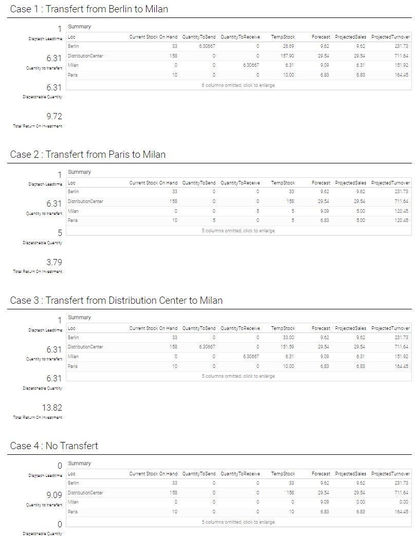
We want to consider here 2 possible types of transfer: a classic transfer from the central warehouse to the agencies and inter-agency transfers. By analyzing the costs associated with the various possible transfers, and using the provided data, identify the best possible solution to reduce the impact of the current stock-out for reference
15343952in Milan.
Hint: Proceed by steps: estimate the needed quantities for the period considered (also called window of opportunity), then the dispatchable quantity, and finally evaluate the return on investment for each potential stock transfer.
2. Conclusion
Overstock
By estimating the appropriate timeframe for each location and determining surplus stock thresholds, CM can effectively identify overstocked products and highlight those incurring the highest costs. This knowledge empowers them to fine-tune stock management and minimize unnecessary overstock investment.
Stock Relocation
Regarding the replenishment strategy for stores, CM is presented with a choice between classic transfers from the central hub to stores or inter-store transfers. This decision has a substantial impact on cost structures and the return on investment of each reference.
These insights underline the value of data-driven decision-making in supply chain management. By aligning stock levels with demand scenarios and making informed choices about transfer strategies, companies can improve significantly operational efficiency, reduce costs, and enhance overall service quality for their customers.
Annex
Get the dataset from the Envision playground
///## 0.1 Reading data tables

/// The list of items, purchased and sold.
read "/Catalog.tsv" as Items[Ref]  with
  /// The primary key, identifies each item.
  Ref : text
  Category : text
  ///Identifies product's supplier.
  Supplier : text
  Brand : text
  /// Unit price to buy 1 unit from the supplier.
  BuyPrice : number
  /// Unit price to sell 1 unit to to a client.
  SellPrice : number

///The list of SKUS, purchased and sold (Reference / Localisation granularity)
read "/SKU.tsv" as Sku[Sku] expect[Ref] with
  /// The primary key, identifies each sku (Reference / Localisation granularity)
  Sku:text
  /// Foreign key to `Items`
  Ref:text
  /// The place where the item is stocked
  Loc:text
  Category:text
  Brand:text
  ///The stock currently available on the shelves (in units)
  StockOnHand:number
  /// Unit price to buy 1 unit from the supplier.
  BuyPrice:number
  /// Unit price to sell 1 unit to to a client.
  SellPrice:number

///The table of past transactions, sold to customer
read "/Orders.tsv.gz" as Orders expect[Ref,Sku,Date]  with
  ///The identifier of the sales transaction
  OrderId : text
  ///The date when the sales orders happened
  Date : date
  /// Foreign key to `SKU`.
  Sku : text
  /// Foreign key to `Items`.
  Ref : text
  /// Where (Localisation) the sale took place
  Loc : text
  ///The quantity delivered to the customer
  DeliveryQty : number
  NetAmount : number
  ///The identifier of the customer
  Client : text
  ///The channel used by the customer for the sales transaction
  SalesChannel : text

/// The list of purchase orders with external ones requested to suppliers and internal ones related to trasnfert
read "/PurchaseOrders.tsv" as PO expect[Ref,Date] with
  /// Identifies the purchase orders, that may include several lines.
  PONumber : text
  /// The date when the PO was originally placed.
  Date : date
  /// Foreign key to `Items`.
  Ref : text
  /// The date when the PO was delivered. : the date `2001-01-01` indicates that the PO hasn't been delivered yet
  DeliveryDate : date
  /// The quantity, in units, originally ordered for the item.
  OrderQty : number
  /// The quantity, in units, finally delivered for the item.
  DeliveryQty : number
  /// The price to be paid to the supplier for this PO line.
  NetAmount : number
  /// When `true`, there is nothing left to be delivered.
  IsClosed : boolean
  /// Purchase Order Type
  Type : text
  /// Localisation of origin (useful for transfers)
  OriginLoc : text
  /// Reception Localisation
  DestinationLoc : text

/// The stock history, per day, for each Sku
read "/StockHistory.tsv" as StockHistory expect[Ref,Sku,Date] with
  ///Date of stock snapshot
  Date : date
  /// Foreign key to `SKU`.
  Sku : text
  /// Foreign key to `Items`.
  Ref : text
  /// Reference the storage location
  Loc : text
  Category : text
  /// On-shelf stock, at a given date
  StockOnHand : number

/// Weekly forecast table for each SKU
read "/WeeklyForecast.tsv" as Forecast expect[Ref,Sku,Date]  with
  ///Corresponds to the Monday of the week in question
  Date : date
  /// Foreign key to `SKU`.
  Sku : text
  /// Foreign key to `Items`.
  Ref : text
  Loc : text
  /// Sold quantities for a given Sku and week
  Sales : number
  ///Estimated average demand for the week in question
  Forecast : number

///## 0.2 Creating data tables

table TransfertInfo = with
  [| as Loc1, as Loc2 , as TransfertLeadtime, as UnitCost|]
  [| "Paris", "Milan" , 1, 2.5|]
  [| "Berlin", "Milan" , 1, 1.75|]
  [| "Berlin", "Paris" , 1, 1.75|]
  [| "DistributionCenter", "Paris" , 1, 1.1|]
  [| "DistributionCenter", "Berlin" , 1, 1.1|]
  [| "DistributionCenter", "Milan" , 1, 1.1|]

show label "SC Structure Analysis" a1g1 {textAlign: center ; textBold: "true"}

show markdown "Generic Documentation" a2g2 with """
  Hi there, welcome to your third Envision exercise! In this exercise, you will dig into the company's data to understand its distribution network.
  You will then further analyze the current and past stock levels to suggest decisions that would be beneficial to the business.
  """


///## 0.4 Displaying raw Data tables

show table "Items" a3  with
  Items.Ref
  Items.Category
  Items.Supplier
  Items.Brand
  Items.BuyPrice
  Items.SellPrice

show table "Sku" b3  with
  Sku.Sku
  SKU.Ref
  Sku.Loc
  Sku.Category
  Sku.Brand
  Sku.StockOnHand
  Sku.BuyPrice
  Sku.SellPrice

show table "Orders" c3  with
  Orders.OrderId
  Orders.Date
  Orders.Sku
  Orders.Ref
  Orders.Loc
  Orders.DeliveryQty
  Orders.NetAmount
  Orders.Client
  Orders.SalesChannel

show table "PO" d3  with
  PO.PONumber
  PO.Date
  PO.Ref
  PO.DeliveryDate
  PO.OrderQty
  PO.DeliveryQty
  PO.NetAmount
  PO.IsClosed
  PO.Type
  PO.OriginLoc
  PO.DestinationLoc

show table "StockHistory" e3  with
  StockHistory.Date
  StockHistory.Sku
  StockHistory.Ref
  StockHistory.Loc
  StockHistory.Category
  StockHistory.StockOnHand

show table "Forecast" f3  with
  Forecast.Date
  Forecast.Sku
  Forecast.Ref
  Forecast.Loc
  Forecast.Sales
  Forecast.Forecast

show table "TransfertInfo" g3  with
  TransfertInfo.Loc1 as "Loc1"
  TransfertInfo.Loc2 as "Loc2"
  TransfertInfo.TransfertLeadtime as "TransfertLeadtime"
  TransfertInfo.UnitCost as "UnitCost"

///## 0.5 Documentation
/// The public Envision documentation is available here: https://docs.lokad.com/

///===============================================================================================///